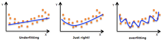
Validation and Evaluation | Applied Machine Learning

Underfitting and overfitting

For explaining underfitting and overfitting, we should first talk about two other concept: variance and bias. We want to avoid high variance and high bias.
A model with a high variance is like a student that memorizes his textbook so literally that he fails to generalize the concepts and answer questions that are slightly different from the examples in his text book.
Variance is how much the your model changes with each training sample. In other words, it shows how much the model is following the pattern of training data.
When the variance of the model is high, we say the model is overfit. The model resembles the training data so much that it fails to make good predictions with new data.
A model with a high bias is like the student reading the textbook so carelessly that he ignores important points here and there. He will fail the exam because of not learning the textbook well.
When the bias of the model is high, we say the model is underfit.
Whereas a high variance means that the model is following the pattern in data too strictly that it fails to generalize, a high bias means the model is following the pattern in data too loosely that it fails to capture it.

Fixing underfit models

Collect more features.
Add polynomial features.
Decrease regularization parameter λ to make the model more complex.

Fixing overfit models

Get more training data.
Try fewer features.
Increase regularization parameter λ to make the model simpler.

Determining overfitting vs underfitting

To test the performance of a model, we need to test it on some data it has never seen before.
That is why we divide the data into two subsets: training set and the test set.
There is no hard rule for what fraction of the data should test, but a common decision is to keep 20% to 30% of the data for testing.
If the model performs well on the training set, but poor on the test set, then it has high variance (overfitting).
If the model performs poor on the training set as well as the test set, it has high bias (underfitting).
But how should we determine the correct number of features or the correct algorithm parameters?
We train the model with each parameter combination and calculate its performance on the test set.
Then we compare the model performances with different parameter combinations and choose the one that results in the best performance on the test set.
So your algorithm is trained with the training set (which ~70% of the data you have), and then its performance is assessed with the test set, data it has never seen before.
You choose the model parameters and number of features so that the algorithm works well for both the training set and the test set.
But it can performs poorly with new data. Why?
The reason is that your algorithm can still suffers overfitting because model parameters were optimized with the test set, and the test set may not be a good representative of new data.

Cross-validation set

To fight back overfitting, we should split our data into three sets.
- One set for training (~60% to 70% of the data)
- A cross-validation (CV) set that we use to tune model parameters, feature sets, etc.
- A test set that the model has never seen, and it never used for tuning model parameters.
There is a problem with the above data segmentation approach. We usually do not have enough data. Only 60% of the data to train our models may be too little. Thus, alternative approaches have been devised.:

Leave one out

In this approach, you do not keep a fixed fraction of the data for CV, instead, you train your model on all training data (i.e., all data except test set) minus one single sample.
You evaluate your model with that single sample put aside.
You repeat the process again but you choose a different sample to evaluate the model.
In the end, your models performance will be the average performance of all the models.
This approach has the advantage that we will use all the data for training our model.
A major problem is that it takes a lot of execution time. We slow-to-train algorithms, or very large dataset, this may not be a feasible option.

K-fold

K-fold CV is different from leave one out in that we first shuffle the data.
Next, we split the data into K segments (folds).
Then, we train our model with leaving one fold out at a time.
The model performance will be the average performance of the models.
This approach leads to way fewer models to train, as K is usually around 3-10.
The exact value of K depends on your data size. It should be large enough to be a representative of the larger data.
It is important that data preparations, such as feature scaling, be applied independently to each K-1 fold of data. Otherwise, we may have “data leakage”, a situation where we use information for training the model that are not in the training data.

Stratified

This is similar to K-fold, except that the proportion of data, according to some condition that we decide, is similar within each fold.
This is important when your data are skewed.

Using CV for diagnosis

A useful plot for diagnosing your model is the one below:

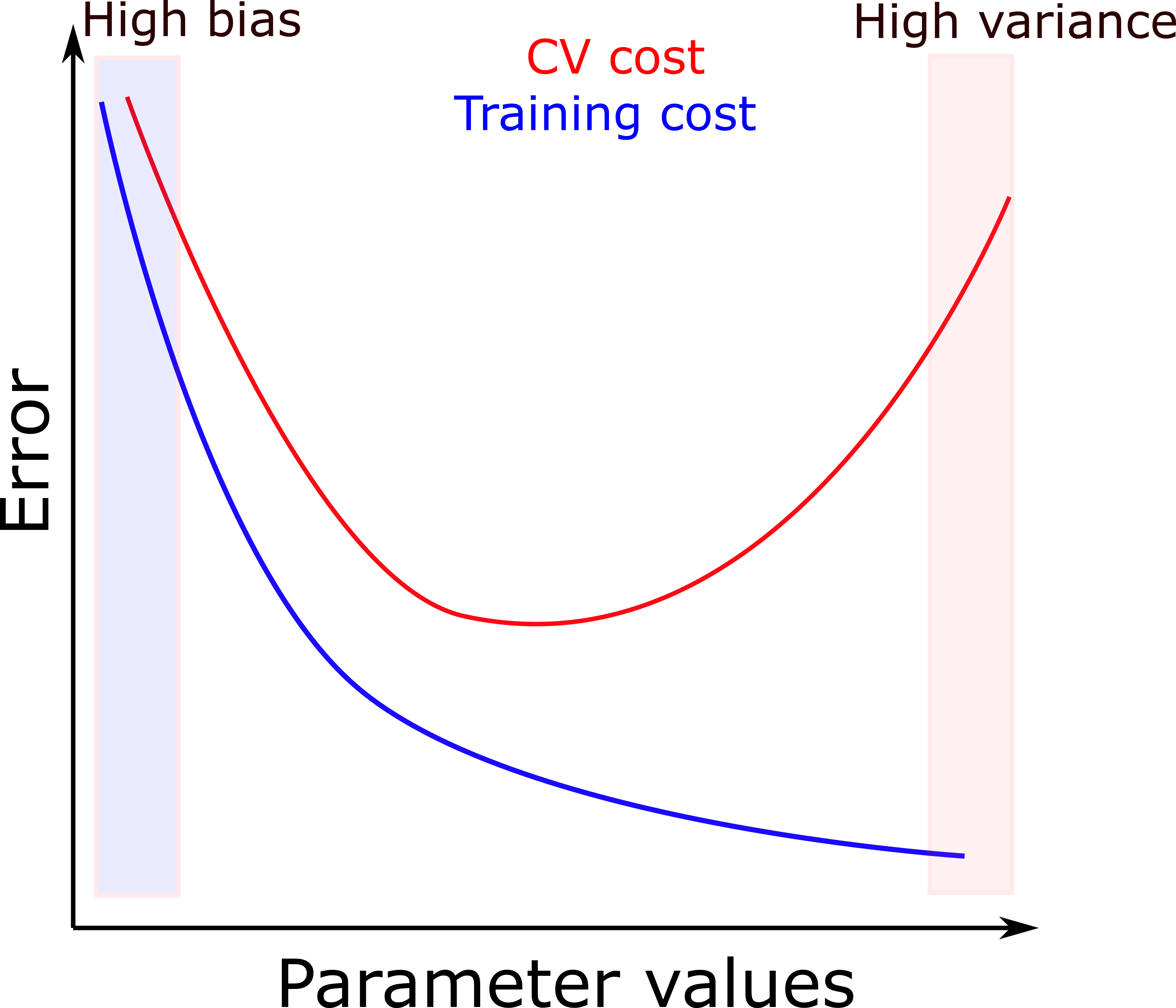
If both the CV set and the training set have high error, then your model suffers from underfitting.
If the training set has low error but CV set has high error, it suffers from overfitting.
The right choice of model parameters is where the CV set and the training set both have low error.
Note on choosing the right regularization parameter λ:
1. Try a range λ values on the training set and for each one of them calculate the training set error.
2. Predict CV test with each trained model and calculate its error. Here, you do not need to use λ as it was only for training.
3. Choose a model with the lowest error on both CV and training set.
4. Report your models performance by calculating its error on the test set.
It is a good idea to choose samples for the test set that you think your machine learning algorithm will ultimately see.
Since your algorithms are focused on improving the CV set, it is important that the CV and test sets both come from the same distribution. Otherwise, your algorithm may work well on the CV set, but not on the test set.
Moreover, when the CV and test sets are from the same distribution, you can diagnose problems easier. If the algorithm works well on the CV but not on the test set, it is a sign that it is overfitting. So you should collect more samples for the CV set.
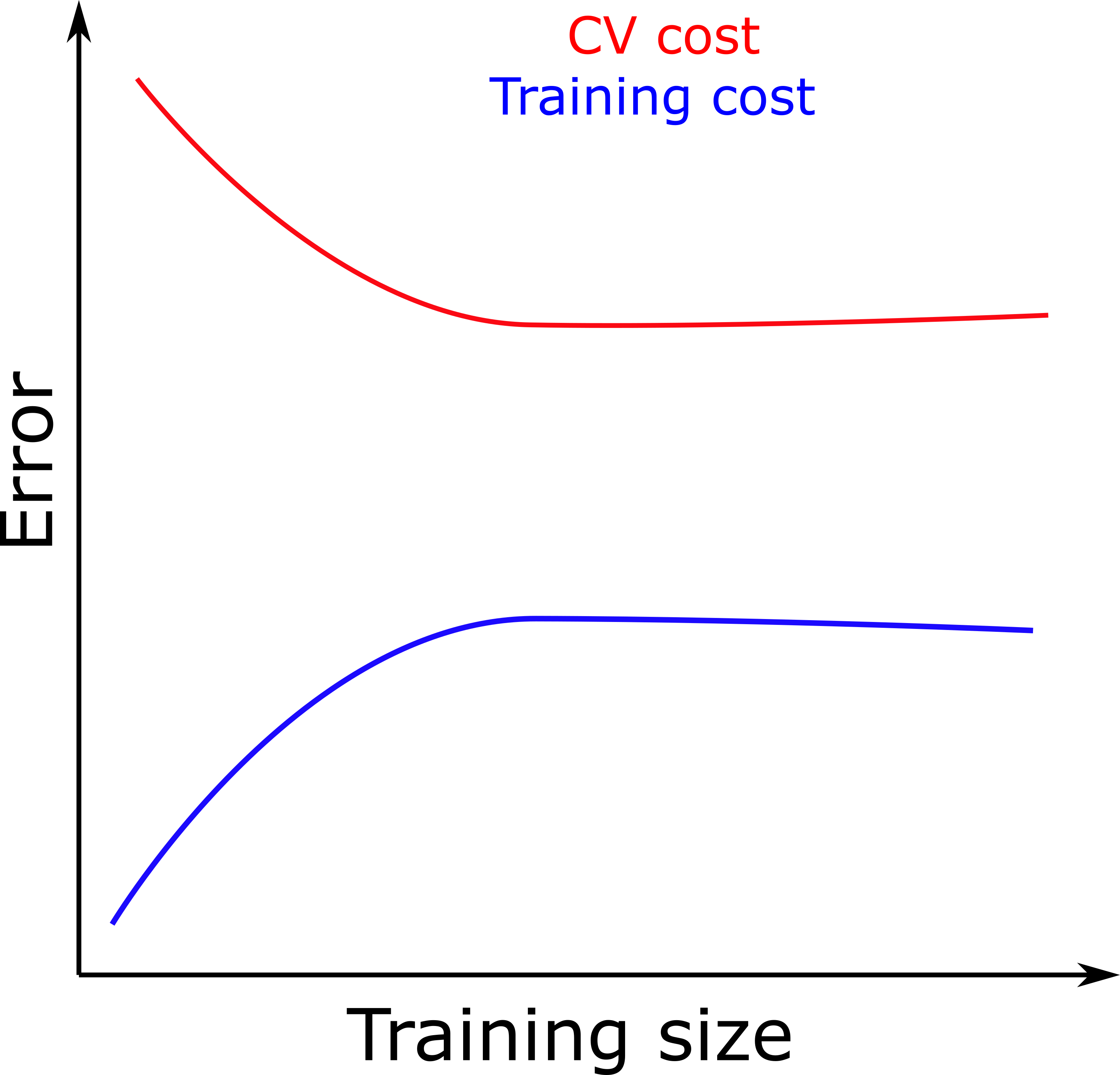
Another plot that is useful for diagnosing the model is a learning curve.
- Building a learning curve is an iterative process.
- We start with a small number of training samples, say one sample for this example.
- We train the model and calculate the training set and CV error.
  - At this state, sinse there is only a single sample, the training model will have error zero because any model can perfectly fit a single point.
  - On the other hand, the CV set will have a large error, because there is not much to generalize from a single point.
- Next, we make the training sample slightly larger, say 10 sample, and repeat the training and calculating errors of training set and CV set.
- We repeat this until our training size equals the number of all our training data.
- We plot the change in CV and training set error against sample size.
- If our model is performing well, we should expect a plot similar to the one below. Of course, it will never be so perfect, all data have noise.

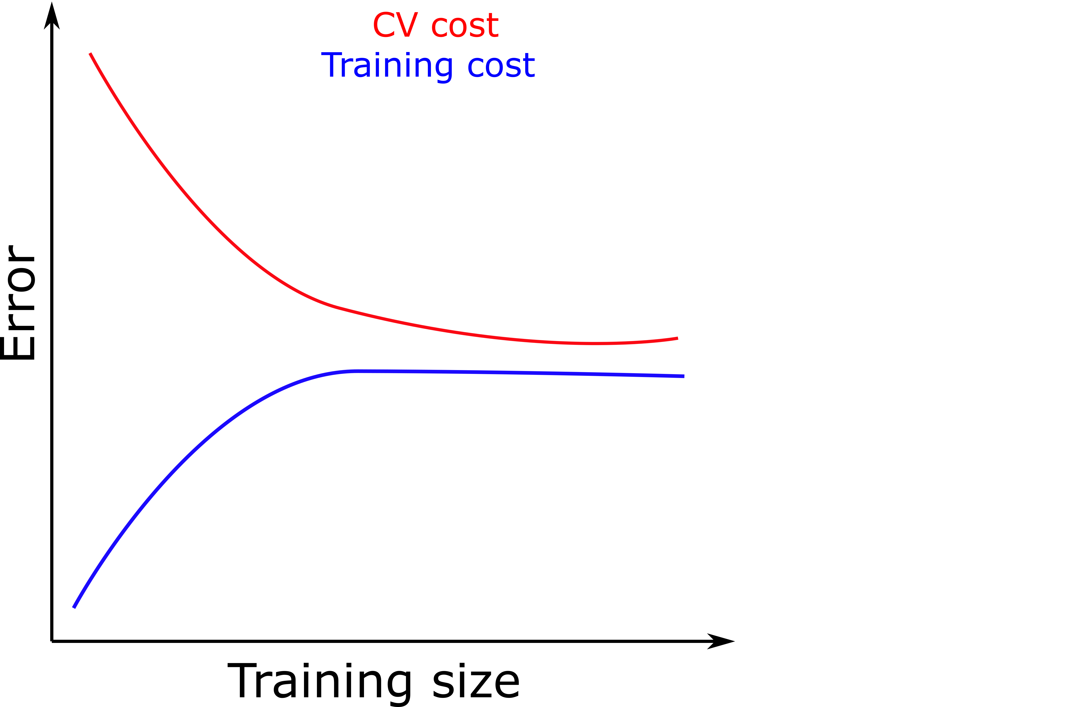
The plot shows that both training set and CV set error keep converging as we add more data until we reach a plateau.
If we do not see a plateau, it is a sign that adding more data will still reduce the CV error, i.e., we are overfitting.
If training and test error are both high and similar (figure below), we are underfitting.

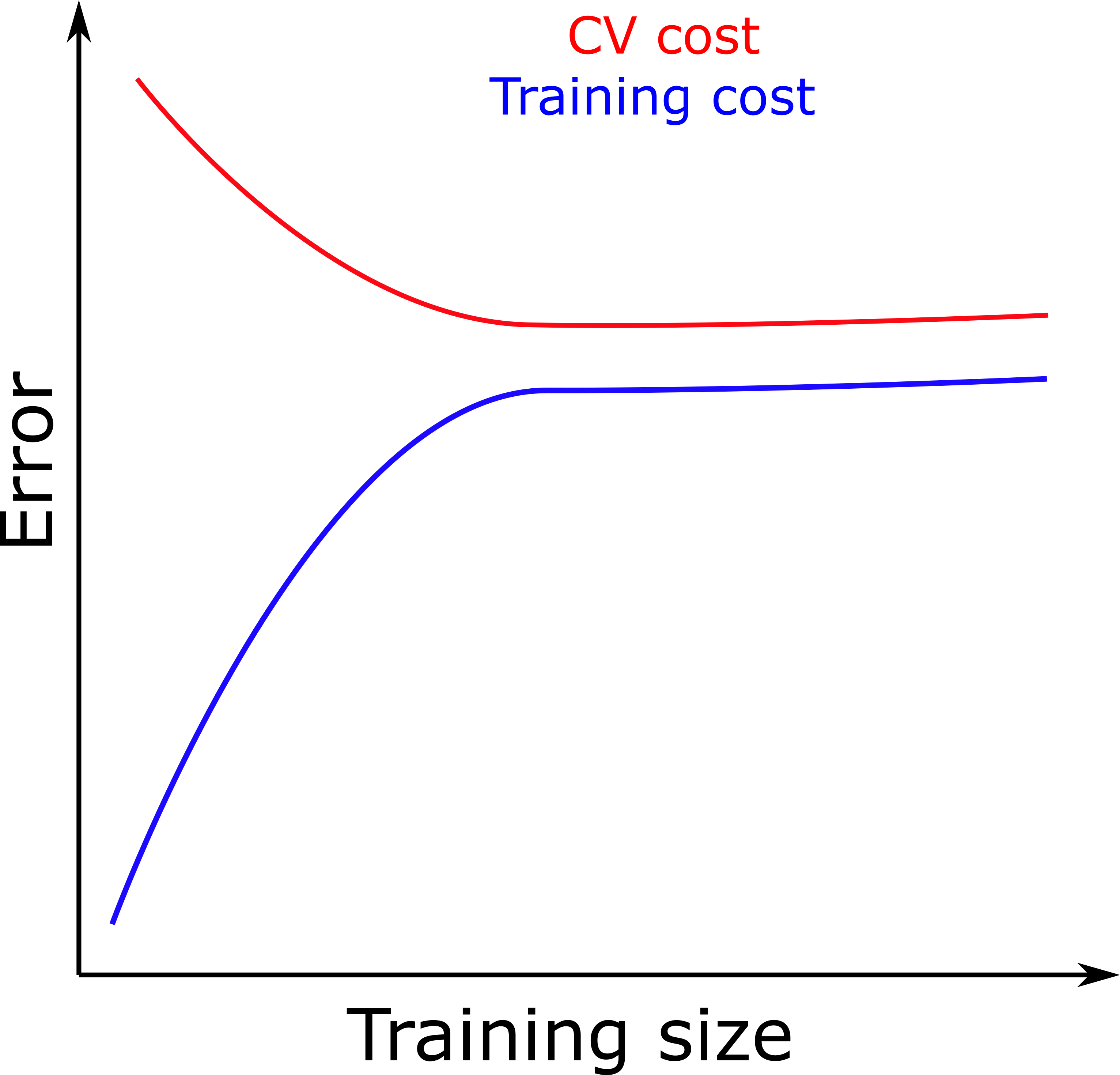
If the difference between the CV set and training set is large (figure below), this means we are overfitting.

Model assessment

After we have collected data and chosen which machine learning algorithms to choose, we need a metric to compare the algorithms against one another.
There are various metrics for regression and classification algorithms, each one of which has its own strengths and weaknesses. The choice of the metric depends on our goal and data.

Classification metrics

All classification metrics perform some operations on confusion matrix.
A confusion is a 2 by 2 matrix that shows the number of true positives, true negatives, false positives, and false negatives.

		Actual
		Positive	Negative
Predicted	Positive	TP	FP
Predicted	Negative	FN	TN
	Total	P	N

The fraction of different parts of the matrix with respect to one another, makes different metrics.

Accuracy

\[\text{accuracy} = \frac{TP + TN}{P + N}\]
Shows closeness of predictions to the target.
In other words, if the average prediction can correctly determine the true response.
Usually, a dataset does not have equal number of positive and negative results. This can be misleading with some metrics, such as accuracy.
For example, the prevalence of breast cancer is 1% and 99% of people are healthy. We develop and algorithm to detect healthy people. The data that we have gathered is a reflection of true distribution of people with cancer. So if we develop the algorithm to only correctly determine true response (healthy and cancer), the algorithm may classify all cases as healthy because it scores well with that classification. Say, we feed it with 1’000 samples, 10 of which have cancer can the algorithm classifies all as healthy. Then the accuracy is 99% (TP=990, FP=10, FN=0, TN=0).

Precision/positive predictive value

\[\text{precision} = \frac{TP}{TP + FP}\]
Shows closeness of predictions to each other.
In other words, it shows the fraction of positive predictions that we truly positive.
This is also not a comprehensive metric, as we have precise but inaccurate predictions.
Say, we want to detect whether there is a person in a picture. Our 1’000 samples are mostly with people in them (900). If our algorithm correctly detects half of the pictures with a person in them (TP=450), does not detect the other half (FN=450), at worst, its precision is 82% (if it incorrectly detects people in all pictures without a person - FP = 100). At best, its precision is 100% (if it correctly does not detect people in the 100 pictures without a person in them - FP = 0).

Recall/sensitivity/true positive rate

\[\text{recall} = \frac{TP}{P}\]
Recall is a complement of precision. It shows the fraction of positive predictions among all truly positive samples.
In the example above, recall is 50%, regardless of how the algorithm detects negative samples.
Recall is sensative to bias in samples in a similar way as accuracy. In the example of detecting healthy people among those who have breast cancer, recall=100%.

F1 score

\[F1 = 2 \frac{\text{recall} \times \text{precision}}{\text{recall}+\text{precision}}\]
It is a combination of precision and recall through harmonic mean, and is generally a better metric than either of them.
This does not mean that we should always choose F1 over recall or precision. The choice should ultimately be made with regard to our goal.

Specificity/true negative rate

\[\text{specificity} = \frac{TN}{N}\]
The fraction of correctly predicted negatives among all negatives. It is a counterpart of recall for negative results.
The focus of specificity is on correctly detecting negative results, so it should be used in cases where finding negatives is more important than finding positives. For example, our algorithm that classifies all samples as healthy, has 0% specificity.

Informedness

\[\text{informedness} = \text{recall} + \text{specificity} - 1\]
Calculates the probability that our prediction is not random.
It takes into account both the fraction of false positives and false negatives.

Regression metrics

Mean Squared Error (MSE)

\[\text{MSE} = \frac{1}{n}\sum_{i=1}^{n}(y_i - \hat{y}_i)^2\]
This is one of the simplest metrics, but is very sensative to outlier.
A single bad prediction has large effect on the metric, because arithmatic mean is sensative to large numbers, and we are squaring differences between actual and predicted values.

Root Mean Squared Error (RMSE)

\[\text{RMSE} = \sqrt{\text{MSE}}\]
An advantage of RMSE to MSE is that the it has a similar scale of errors as the actual data.
An other advantage is that outlier residuals do not affect the metric as much.
RMSE is similar to MSE in that they are directly comparable. If MSE of a algorithm A is larger of that of algorithm B, we are show that their RMSEs have the same relationship.

Mean Absolute Error (MAE)

\[\text{MAE} = \frac{1}{n}\sum_{i=1}^{n}\|y_i - \hat{y}_i\|\]
Since MAE does not square the residuals, it is less sensative to large residuals than MSE and RMSE.
A problem with MAE is that it is not differentiable when the prediction is perfect.

\(R^2\)

\(R^2 = 1 - \frac{\text{MSE}}{\text{MSE (baseline)}}\), where \(\text{MSE (baseline)} = \frac{1}{n}\sum_{i=1}^{n}(\bar{y} - \hat{y}_i)^2\)
Called the coefficient of determination, it provides a scale-free metric with a maximum of 1. So we can have a sense of how good a model is.
When \(R^2 < 1\), the predictions are worse than predicting the mean of all samples (the simplest model).

General advice

Although each metric has its own weaknesses, but choosing a single metric to compare all your models will help decision making
If you need to satisfy multiple criteria which cannot be combined into a single metric, here is good solution. With N criteria, choose only one criteria to maximize your algorithms. But also choose minimum values for other N-1 criteria. So your algorithm maximized on one metric, but has to be good enough with respect to other metrics.
If your algorithm performs against what you expect, maybe the metric you have chosen is not a good one. In that case, think about a new one. It may also be because your test set is not a good representative of data.
It is a good idea to always start building your model from simple ones to more complex ones if needed. Sometimes, a simple algorithm can perform better than or on par with more complex ensemble ones. That is why the simpler algorithms are not obsolete. Another advantage is that starting from simpler scenarios, you can quickly get an intuition of the structure of the data, and areas you need to focus.

Example workflow

Here is an example of using cross validation and parameter search using Scikit-learn.

using ScikitLearn
@sk_import neighbors: KNeighborsClassifier
@sk_import model_selection: StratifiedKFold
@sk_import metrics: f1_score
@sk_import datasets: load_breast_cancer
@sk_import model_selection: GridSearchCV
@sk_import preprocessing: PolynomialFeatures
@sk_import preprocessing: RobustScaler
@sk_import model_selection: train_test_split

all_data = load_breast_cancer()
X = all_data["data"];
y = all_data["target"];

X_train, X_test, y_train, y_test = train_test_split(X, y, train_size=0.8)


"""
Add polynomials to features to your data.
"""
function addpolynomials(X; degree=2, interaction_only=false, include_bias=true)
  poly = PolynomialFeatures(degree=degree, interaction_only=interaction_only, include_bias=include_bias)
  fit!(poly, X)
  x2 = transform(poly, X)
  return x2
end

function KNN_classification(X_train, y_train; nsplits=5, scoring="f1", n_jobs=1, stratify=nothing)

  # Scale the data first
  rscale = RobustScaler()
  X_train = rscale.fit_transform(X_train)

  # build the model and grid search object
  model = KNeighborsClassifier()
  parameters = Dict("n_neighbors" => 1:2:30, "weights" => ("uniform", "distance"))
  kf = StratifiedKFold(n_splits=nsplits, shuffle=true)
  gridsearch = GridSearchCV(model, parameters, scoring=scoring, cv=kf, n_jobs=n_jobs, verbose=0)

  # train the model
  fit!(gridsearch, X_train, y_train)

  best_estimator = gridsearch.best_estimator_

  return best_estimator, gridsearch, rscale
end

### Use the function
######################

best_estimator, gridsearch, rscale = KNN_classification(X_train, y_train)

# Make predictions:

# transform X_test
X_test_transformed = rscale.transform(X_test)

y_pred = predict(best_estimator, X_test_transformed)

# Evaluate the predictions

f1_score(y_test, y_pred)

## learning for model evaluation

@sk_import model_selection: learning_curve 

cv = StratifiedKFold(n_splits=nsplits, shuffle=true)
train_sizes, train_scores, test_scores = learning_curve(best_estimator, X_train, y_train, cv=cv, scoring="accuracy", shuffle=true)