Data preparation | Applied Machine Learning

Data scientists collect data from different sources, such as experimental and observational studies, and data scrapping.
In most cases, data need to be cleaned and converted to a desired format before analysis.
Here, we talk about data manipulation in data frames and different methods of handling files.

Data Frames

DataFrame (DF) format, which organizes data in tables is a cornerstone for data analysis in Julia.
DFs are used when data is not homogeneous, i.e., data samples have with different formats or there are missing or incomplete values. If it were homogeneous, lists and matrices would suffice.
DFs also ease “data cleaning”.
Data preparation is often the most time-consuming task in machine learning.
We will clean a dataset using the DataFrames package and with that, demonstrate some basic concepts.

Useful functions

From the DataFrames package: first, last, names, show, size. describe.
ismissing, unique, skipmissing, dropmissing.

Data types

All variables can be categorized as either numerical or categorical.
Any variable that involves some measurement is numerical. Examples include temperature and speed.
Any variable that categorizes or groups information is categorical. Examples include colors, gender, and people names.
Categorical variables can be further divided to two classes: nominal and ordinal.
Nominal variables are no order with respect to one another. “Male” and “female” are two categories of gender and there is no intrinsic ordering between them.
Ordinal variables, on the other hand, have a clear ordering. For example, classifying employees’ performances as “good”, “medium”, and “poor” can be ordered.
Note that the interval between different ordinal categories may not be equal.
If the difference between ordinal variables is fixed, then we have and interval variable.
Why does it matter to determine data types? because certain operations do not make sense on all data types. You can not take the mean of some colors, or taking the mean of an ordinal data with unequal intervals is problematic.

Handling missing values

There are different approaches for handling missing data. Choosing an approach depends on your data (e.g. how many missings there are), and on your objective.
Making the right decision is sometimes a challenging task and can determine the performance of your ML code.

Deleting

This is the most intuitive approach. When a row has a missing value in some columns or a column has many missing values, we just remove those rows/columns.
This method works when there is a large number of samples and removing some of them does not impact your ML model performance.
When a large fraction of the data (e.g. ~30%) is missing, removing them is not a good idea.

Replacing with a summary statistic (imputation)

This method is suitable for numerical data.
It involves replacing the missing values with a summary statistic of the non-missing data, such as mean, median, or mode.
The logic is that we approximate the missing values from the non-missing ones.
It can introduce some error to the data, but the error can have less detrimental impact on the ML model than removing the missing rows altogether.
This method is suitable when sample size is small.

Assigning a new class

Good for categorical data.
Involves adding a new category for the missing data.
A downside is that the extra category can negatively impact the model performance.

Prediction

We can create a machine learning model using the non-missing values, and then predict the missing ones with that model.
This method introduces less error into the data than replacing the missing values with summary statistics.

Using ML algorithms that support missing values.

Some ML algorithms work even if there are missing values.
Examples are K-nearest neighbors and random forests.

Feature scaling

When you have multiple features (input columns), it is important to make sure they are on the same scale. If data are not within the same scale, gradient descent will be very slow and the predictions become poor.
There are different ways to scale features, and choosing one depends on the structure of your data and the machine learning model you are going to use.
Feature scaling is essential for machine learning algorithms that calculate distances between data, such as regression and K-nearest neighbors. Without scaling, features with larger values are given more importance.
Machine learning algorithms that do not use distance between data (e.g. Naive Bayes and tree-based methods), do not require scaling.

Mean normalization

Puts each sample between -1 to 1.
Formula: $\frac{x_i - \mu(x)}{maximum(x) - minimum(x)}$.

Standardization or Z-score normalization

The goal is to redistribute the data such that they have a mean of 0 and standard deviation of 1.
Assumes your data is normally distributed.
Procedure:
1. Calculate the mean and standard deviation for each feature.
2. Change each sample of the feature using the following formula: $\frac{x_i - \mu(x) }{\sigma(x)}$, where $\mu(x)$ is feature mean and $\sigma(x)$ is feature standard deviation.

Min-Max normalization

One of the most commonly used scaling algorithms.
Puts all samples in the same range: 0 to 1 if there are no negative numbers, or -1 to 1 if there are negative numbers.
Scale each sample using the following formula $\frac{x_i - minimum(x)}{maximum(x) - minimum(x)}$.
If data are not normally distributed or the standard deviation is too small, use this scaler.
This scaling method is sensitive to outliers. Check if you have outliers before using it.

Handing categorical variables

Challenges with categorical features:
- We cannot input raw categorical variables into many machine learning models, such as regressions. Most ML models need numerical data.
- Categorical variables may have too many categories, which reduce the performance of a model. For example, ZIP code of houses is a categorical features that may be used for predicting rent prices, but with so many ZIP codes, it may negatively affect the model.
- Some categories rarely occur. Therefore, making correct predictions for them is difficult.

One-hot encoding

For nominal variables.
For each category of a categorical feature, create a new feature.
The new features are binary, only accepting 0 or 1.
Within each new feature, all samples are 0 except those that belong to a single categry.
Example:
- We have a feature for people who like cats or dogs or both. So the feature has three categories: “cat”, “dog”, and “both”.
- We create a new feature for each category. For cats, only the cat people will receive a 1, and people who like dogs or both will receive a 0.
- A second feature is created for dogs. Dog people receive a 1 and the rest receive 0.
- We do not need a third feature for “both”, as two zeros for cat and dog implies a third option.
- So in general, we need N-1 new features, where N is number of categories
One downside of this encoding is that if your features have mean categories, you will end up with too many new features that can cause memory problems.
The other downside is that one-hot encoded data are difficult for tree-based algorithms (e.g. random forests) to handle.

Label encoding

For ordinal variables.
This is simpler than One-hot encoding.
It gives each category an integer.
For example, if we have a feature of student performances as “good”, “medium”, and “poor”, we can convert them to 3, 2, 1.
Note that in this case, the algorithm assumes an order between the categories, that is, good (3) is more than medium (2) which is more than poor (1).

Binary encoding

This is an alternative to one-hot encoding that results in fewer new features.
The downside is that some information is lost because close values share many of the columns. So only use binary encoding if there are many categories in a feature.
It works for nominal features.
Algorithm:
1. Assign an integer to each category, starting from 1 to N, where N is the number of categories. The order does not matter.
2. Convert each integer to its binary representation. For example, number one in binary is 01, and number 2 is 10. You can use the function Base.bin to convert a number to its binary representation: Base.bin(UInt(3), 1, false). The number of digits in a binary representation increases for larger integers. It is a good idea to first convert your largest integer, see how many digits it has, and then assign that many “padding” to smaller numbers. For example, say the largest integer is 100. Base.bin(UInt(100), 1, false) returns 1100100, which has 7 digits. For all other integers smaller than that, we use padding 7. For number 1, it will be Base.bin(UInt(1), 7, false) which returns 0000001.
3. Each digit in your binary numbers will be one column/feature. If you used one-hot encoding for a feature with 100 categories, you would have 99 new features. But with binary encoding, you will have only 7 new features.
4. Note that Base.bin returns a string. Convert each single digit of the binary numbers to an integer before putting them in your table.
5. Alternative to Base.bin, you may use string(<integer>, base=2).

Feature selection

It your model is too complex (overfits), one way to reduce its complexity is to choose a set of features that best represent the data without losing too much info.
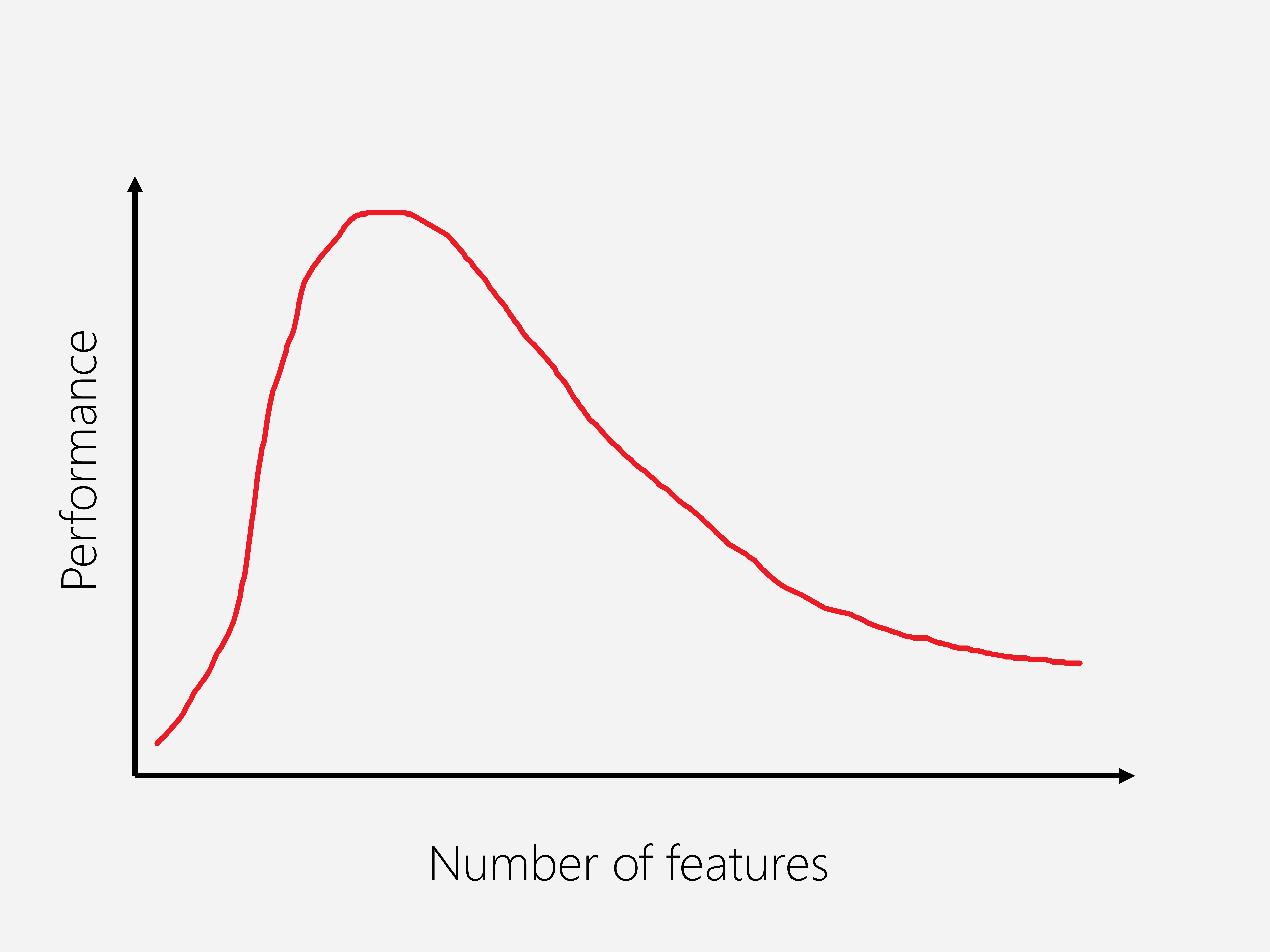
The need for an optimum number of features is referred to as the “curse of dimensionality”. Briefly, it states that the more dimensional our data, the more samples we need to maintain the same level of model performance. The number of needed samples increase exponentially with increasing the dimensionality of data.

Another reason for selecting a subset of features is improving the speed of an algorithm.
There are many different approaches to choosing a set of features, e.g., PCA, variable ranking, and non-negative matrix factorization (NMF).
If you use dimensionality reduction methods, such as PCA, you do not select a subset of features, but create new features.
The criteria for finding the optimum number of features is often a predictors performance.

Ranking method

Go through each feature and apply a scoring function to it. Sort the features by their scores. Choose the top k features, or features with a minimum score in percentage.
This is a simple and fast to perform approach, but the results it provide are not optimal.
A scoring function can be Correlation: the more a feature is correlated with the target, the higher score it has. Correlation may be computed using Pearson correlation coefficient. Since Pearson correlation coefficient ranges between -1 and 1, it is good idea to use the absolute value of the coefficient, not to lose features with negative correlation.
Note that sometimes a feature with a small correlation to the output can be useful with other features. So it is not easy to discard any feature with a small score. So covariance between pairs of features should be considered as well, but it makes the analyasis difficult.
Scikit-learn provides some handy functions for this kind of analysis: SelectKBest and SelectPercentile.
Some other scoring functions include chi square test (chi2 function in sklearn) for classification and univariate linear regression (f_regression function in sklearn) for regression problems.
Another scoring function can be the performance of a machine learning model using only one variable.

Removing low variance features

Features with variance of zero or a very low variance, may be removed.

In Scikit-learn:

using ScikitLearn
import ScikitLearn: fit!, predict
@sk_import feature_selection: VarianceThreshold

X = rand(15, 10)
Model = VarianceThreshold(0.05)
X_new = fit_transform!(s, X)

Principal Component Analysis (PCA)

PCA determines the most important axis by which data are spread.
It provides a possibly smaller set of features to describe the data, but those features are not a subset of the original features.
Each of the principal components describe a mix of the original features. So the new features do not have a direct meaning.

Using machine learning models

Many machine learning models produce a list of feature importances. For example, the coefficients of a linear model, or the priorities of a decision tree are proxies of feature importances.
We can fit all the data to one of those models and then remove those features with smallest importances.
In Scikit-learn, any algorithm with a field feature_importances_ or coef_ can provide that data.

Exercises

Open the datasets below and explore the variables. Select one categorical and one numerical feature from each dataset. Format the selected features to the appropriate form. For example, handle the missing values. Should they be removed? or replaced with a summary statistic? What would you do about the categorical variable? Is it nominal or ordinal? Which procedure is best to convert it to a proper form?

Datasets

Dataset 1: Use the hotel bookings dataset (from kaggle) to define a set of clean features that may be used to predict when hotels receive high demand. It may be useful for planning a trip to get cheapest stay costs.
Dataset 2: This dataset lists project data available from the US Governments IT Dashboard system. It covers the projected and actual costs and timings of a number of government funded projects in the US. Download (from theodi.org). Create a new dataset with a set of clean features that may be used to predict “Projected/Actual Cost ($ M)”.
Dataset 3: UK GP Earnings. This dataset lists earnings data for medical doctors in the UK from 2009. Download: Download (from theodi.org). Create a new dataset with a set of clean features that may be used to predict “Effective_Returns”. (optional)
Dataset 4: This dataset lists the statewide and multi-parish elected officials, all elected officials in a parish, and all elected officials in an office Download (from theodi.org). (optional)