This tutorial is for people who have a basic exposure to programming. It is a compendium of several tutorials1 and the official documentation.
The REPL
When you type julia in the terminal or command prompt, or just click on the Julia icon, you enter the REPL (Read/Evaluate/Print/Loop). This is an interactive environment where you can test your code and get immediate results printed on screen. The REPL is very useful for testing each expression that so make sure it does what you expect. But the code should be written in a text editor or IDE so that you can save it to a file and use it later.
To use the REPL, write some code and press enter. The result will be printed below it:
julia> print("this is some test")
this is some test
When the result takes a lot of space and you do not want it printed on the screen, add a semicolon ; at the end of the line and it will not be printed:
julia> print("this is some test");
julia>
Getting help
To get help about the usage of any function or object, type a question mark ? and the REPL will change to the help mode. There you can type of the name of the object and press enter to get more information about it:
help?> print
search: print println printstyled sprint isprint prevind parentindices precision escape_string setprecision unescape_string process_running CapturedException

  print([io::IO], xs...)

  Write to io (or to the default output stream stdout if io is not given) a canonical (un-decorated) text representation of values xs if there is one, otherwise
  call show. The representation used by print includes minimal formatting and tries to avoid Julia-specific details.

  Printing nothing is not allowed and throws an error.

  Examples
  ≡≡≡≡≡≡≡≡≡≡

  julia> print("Hello World!")
  Hello World!
  julia> io = IOBuffer();

  julia> print(io, "Hello", ' ', :World!)

  julia> String(take!(io))
  "Hello World!"

julia>
A very useful function to get help is apropos. When you do not know the name of the function that does what you want, you can use the apropos to search all the documentations for the keyword you provide. For example, let’s say we want to know how to do dot product in Julia. We simply search the documentation for it:
julia> apropos("dot product")
LinearAlgebra.dot
LinearAlgebra.opnorm
LinearAlgebra.BLAS.dot

julia>
It returns three functions from the LinearAlgebra library that have the word dot product in their documentations. You can then search the documentation of any of the returned functions by preceding it with a ?.
Package mode
To install, update, and check status of packages, just type a right bracket ] in a new line in REPL. You can install any new package with the add command and the package name. This provides a very easy and hassle-free method of downloading and installing packages.
(v1.1) Pkg> add DataFrames
To exit the Pkg mode, press backspace or Ctrl+C in and empty line.
Shell mode
Typing a semicolon ; in a new line take the REPL to the shell mode, as if you had not entered into the REPL: you can type any shell command and see the results.
Some useful interactive functions
edit("pathname"): launch the default editor and open the filepathnamefor editing.@edit rand(): launch the default editor and open the file containing the definition of the built-in function rand()less("filename-in-current-directory"): displays the file in the pager
Tab auto-completion
When you something in the REPL and press tab, any object or function that has the same beginning will show, so you can choose from them. For example, if you write Mat in the REPL and press tab twice, two object names print on the screen: MathConstants and Matrix. If you add r and then press tab again, it will complete the word Matrix for you.
Syntax highlighting
There is no syntax highlighting in REPL by default. But you can get that by installing and using the OhMyREPL package:
(v1.1) Pkg> add OhMyREPL
julia> using OhMyREPL
Typing special characters
To type special characters like the greek letters, type the name of the letter after a slash \ and followed by a tab:
julia> \pi TAB
will print:
julia> π
π = 3.1415926535897...
History
If you have previously types some long lines of code, and you want to run them again, you do not have to type them in again. Just use the Up arrow key to go through your previous command. This history does not get erased after you close REPL.
Syntax
Julia’s syntax will be familiar if you have any experience with Python of Matlab. On this page you can see a comparison of the syntax of the three languages.
Arithmetic operations
- The operators
+,-,*,/, and^perform addition, subtraction, multiplication, division, and exponentiation.
julia> 2 + 3
5
julia> 2 - 3
-1
julia> 2 * 3
6
julia> 2/3
0.6666666666666666
julia> 2^3
8
Strings
A string is a sequence of characters. A character is enclosed in single quotes '' and strings are enclosed in double quotes "".
julia> mystring = "some text"
"some text"

julia> mystring[1]
's': ASCII/Unicode U+0073 (category Ll: Letter, lowercase)

julia> mystring[1:3]  # indexing sub strings
"som"

julia> length(mystring)
9
- Strings are immutable. This
mystring[1] = 't'will not work. - You can concatenate two string using
*:"this" * " is" * " a" * " string." - You can create strings from variables using
$:julia> a = "Julia" "Julia" julia> "I am learning $a" "I am learning Julia" - Strings can be converted to upper case or lower case:
julia> uppercase("some text") "SOME TEXT" julia> lowercase("SOME TEXT") "some text" - Strings of numbers can be converted back using the
parsecommand:julia> parse(Float64, "1.2") 1.2 julia> parse(Int, "2") 2
Arrays and tuples
Arrays are lists of objects. An array can include objects of different types.
An easy way to build an array is to use []:
julia> a = [1,2,3]
3-element Array{Int64,1}:
 1
 2
 3
You can mix different types and even include arrays inside arrays (nested arrays):
julia> b = [1, 1.2, a, "some text"]
4-element Array{Any,1}:
 1
 1.2
  [1, 2, 3]
  "some text"
Note that the type of elements in an array are expressed in its type. For example, since a only contains integers, it is an Array{Int64,1}: an array whose elements are all Int64 and whose dimension is 1 (it is a single column). Since b contains elements with various types, it is Array{Any,1}.
Creating empty arrays of specific types
Generally, arrays of generic types, such as Any, reduce the performance of your program. So it is better to make sure your arrays contain single object types.
You can create an empty array of type Any with []. To create an empty array with a concrete type, precede the [] with the type:
julia> c = Int64[]
0-element Array{Int64,1}
You can then add elements to your array using the push! command:
julia> push!(c, 5)
1-element Array{Int64,1}:
 5
Since c is an array of Int64, you cannot add other types to it:
julia> push!(c, 1.2)
ERROR: InexactError: Int64(1.2)
Stacktrace:
 [1] Type at .\float.jl:703 [inlined]
 [2] convert at .\number.jl:7 [inlined]
 [3] push!(::Array{Int64,1}, ::Float64) at .\array.jl:853
 [4] top-level scope at none:0
You can also create an array and preallocate its size. This can increase your program’s performance.
julia> d = Array{Int64}(undef, 3)
3-element Array{Int64,1}:
 164348592
 259262672
 251929088
To add elements to a preallocated array, use indices:
julia> d[1] = 6
6
julia> d[2] = 7
7
julia> d[3] = 8
8
julia> d
3-element Array{Int64,1}:
 6
 7
 8
Arrays can also be generated from comprehensions:
julia> e = [i for i in 1:10]
10-element Vector{Int64}:
  1
  2
  3
  4
  5
  6
  7
  8
  9
 10
Arrays are stored in memory as columns, not rows.
To access a given element in an array by index, use []:
julia> b[2]
1.2
Arrays are indexed from 1, like mathematical notation, and unlike some languages like C++ and Python.
Finding the index of an element in an array
julia> a = [5,4,3,2,1];
julia> findfirst(a-> a==2, a)
4

julia> a = [5,4,3,2,2,1];
julia> findall(a-> a==2, a)
2-element Array{Int64,1}:
 4
 5
Matrices
- Matrices in Julia are multidimensional arrays:
rand(3,4):julia> a = rand(2, 3) 2×3 Array{Float64,2}: 0.41701 0.223288 0.566576 0.376302 0.523248 7.56314e-5 - They can indexed in all their dimensions:
a[2, 3] # element on the second row and the third column. a[1, 1:3] # first row and columns 1 to 3. a[[1,2], [3,4]] # first and second row in the third and fourth column. - Matrices are column based, meaning that column-wise operations are faster than row-wise operations.
Types
Every data element you work with belongs to a type (shape and size). For example, number 2 is of type integer, and 2.0 or 0.2 are floating point numbers.
Julia is an optionally-typed language, meaning that you do not have to provide the type of variables when you code. However, this can be necessary sometimes as we will see in the future sections, for example, when you want to take advantage of multiple dipatch.
To determine the type of a variable, use the typeof function:
julia> typeof(2)
Int64
julia> typeof(2.0)
Float64
julia> typeof("some text")
String
There is a type hierarchy in Julia; some types are abstract and encompass several other concrete types. For example, the Integer type includes Int64, Int32, Int16, etc. The root of all types is Any. Figure below shows the type hierarchy of numbers in Julia:
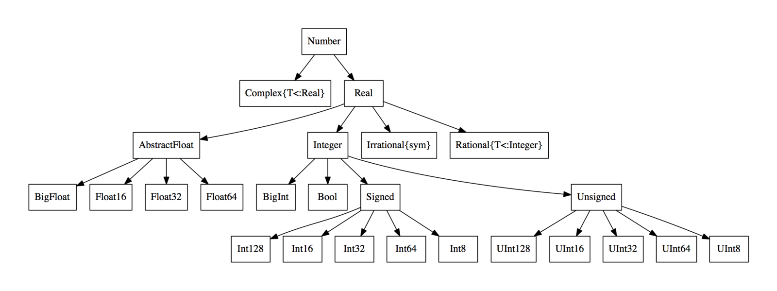
To find the parent of type, use the supertype command. To find all the subtypes of a type, use the subtypes command:
julia> subtypes(Integer)
3-element Array{Any,1}:
 Bool
 Signed
 Unsigned

julia> supertype(Int32)
Signed
Integer and Floating point types
Integer and Floating types have different versions denoted by numbers such as 64, 32, etc. These numbers refer to the capacity of the type, i.e how many digits it can store. An Int64 stores more digits than an Int32. The exact range of numbers representable by each signed (including negative values) integer type can be calculated as following: \(-2^{n-1}\) to \(2^{n-1} -1\). Thus, Int16 covers a range of -32768 to 32767. Unsigned integers are represented by adding a U in the beginning of the integer type, and they only include positive numbers. For example, UInt16 covers \(0\) to \(2^{16} -1 (65,535)\).
Concrete and abstract types
Those types that have children/subtypes are abstract. An abstract type denotes a category, but cannot be assigned to an object. You cannot have an integer of type Number. In other words, the leaves of the type hierarchy tree can be assigned to specific objects.
Numerical type conversion
The notation T(x) or convert(T,x) converts x to a value of type T:
julia> Float64(2)
2.0

julia> Int64(2.0)
2
To convert a number x stored in a string to a number type T, use parse(T, x):
julia> parse(Int64, "32")
32
Defining your own structures
Structures are user-defined types in contrast to the language types such as Int64. These types can have multiple fields, so they are also called “composite types”. They are good tools for grouping a set of values together. “Objects” can be constructed as individual instances of these types.
You can build mutable structures with the following syntax:
mutable struct MyType
  a::Int64
  b::Float64
end
To build immutable types, drop the mutable before the struct. However, mutable fields, like arrays, remain mutable, even in an immutable structure.
- The
a::Bsyntax defines the type of inner fields of a composite type, i.e. a is of type B. - The
a<:Bsyntac specifies that a is a subtype of B. - If you do not define any type for a field, it supports
anytype. But this is not good for speed
An object can be initialized from a structure as follows:
myObject = MyType(2, 2.0)  # the order matters
myObject.a # 2
Control flow
For loops and if statements:
for i in 1:10
  if i%2 == 0
    println(i)
  else
    println(i^2)
  end
end
To stop a a for loop, you can use break.
You can also use list comprehensions:
a = [i for i in 1:10 if i%2 == 0]
a while statement is like a for loop that runs as long as the statement is true:
while true
  println("true")
end
The above code will printn true indefinitely.
Ternary operator
a ? b : c (if a is true, then b, else c).
- The
?and:should have spaces around them.
Logical operators
- and:
&& - or:
|| - not:
!
Functions
Functions can be define with the function keyword:
function f(x)
  x^2
end
Sometimes, it is easier to define them inline:
f(x) = x^2
Arguments of functions are specified by their position. If you want to specify arguments by name, use a semicolon before the list of named arguments:
function g(x, y; z, w=2)
  x+y * z -w
end
When you want to call function g, the first two arguments are x, and y. But for the rest of arguments, order does not matter, and you should provide their names. Node that w has a default value and you may skip passing a value to it.
g(2,3,w=3,z=4) # 11
Multiple dispatch
You can define the same function to handle different types and numbers of inputs. This can be very useful when designing your program. This concept in Julia is called “multiple dispatch”. When you want the function to use different procedures based on the type of inputs, you should specify input types in the function definition:
julia> f(x::Float64, y::Float64) = 2x + y
f (generic function with 1 method)

julia> f(2.0, 3.0)
7.0

julia> f(2.0, 3)
ERROR: MethodError: no method matching f(::Float64, ::Int64)
Closest candidates are:
  f(::Float64, !Matched::Float64) at none:1

julia> f(x::Number, y::Number) = 2x - y
f (generic function with 2 methods)

julia> f(2.0, 3)
1.0
Anonymous functions
Sometimes, you do not need to name a function, e.g. in the map or findall function. In such cases you can use anonymous functions:
x -> x/2

findall(x-> x%2==0, 1:10)
Broadcasting
Broadcasting means applying a function to all elements of an array. In Julia, putting a . after a function name automatically broadcasts it to all elements of its input:
julia> h(x::Integer) = x^2 - 2x
h (generic function with 1 method)

julia> h([1,2,3])
ERROR: MethodError: no method matching h(::Array{Int64,1})
Closest candidates are:
  h(::Integer) at REPL[23]:1
    Stacktrace:
[1] top-level scope at REPL[24]:1
julia> h.([1,2,3])                                                                                                      3-element Array{Int64,1}:
 -1
  0
  3
Dictionaries and sets
- Sets are like lists with two differences:
- They do not keep the order with which values have been added to them.
- They keep only one copy of each element. In other words, all elements in a list are unique.
julia> a = Set([1,1,2,2,2,3])
Set([2, 3, 1])

julia> a[1]
ERROR: MethodError: no method matching getindex(::Set{Int64}, ::Int64)
- A dictionary maps between keys and values:
julia> mydict = Dict()
Dict{Any,Any} with 0 entries

julia> mydict["key1"] = "value1"
"value1"

# define a dict with specific key and value types:
julia> mydict = Dict{AbstractString, AbstractString}()
Dict{AbstractString,AbstractString} with 0 entries

# Predefine a dictionary:
```jl
julia> mydict = Dict{AbstractString, AbstractString}("k1" => "v1", "k2" => "v2")
Dict{AbstractString,AbstractString} with 2 entries:
  "k1" => "v1"
  "k2" => "v2"

julia> mydict["k1"]
"v1"
Function keys returns all the keys of a dictionary, and values returns all the values.
DataFrames
- The DataFrames.jl package is available in Julia package system and can be downloaded with the following command:
]add DataFrames. Start using this package withusing DataFrames. - . Examples below are from the DataFrames.jl’s documentation.
- A
DataFrameis a table of your data, where each column is an array and has its own type. - Constructing a
DataFramefrom arrays:julia> using DataFrames julia> df = DataFrame(A = 1:4, B = ["M", "F", "F", "M"]) 4×2 DataFrame │ Row │ A │ B │ │ │ Int64 │ String │ ├─────┼───────┼────────┤ │ 1 │ 1 │ M │ │ 2 │ 2 │ F │ │ 3 │ 3 │ F │ │ 4 │ 4 │ M │ - Access each column via via
df.colordf[!, :col]ordf[!, 1]. names(df)returns column names.- To add columns to an empty DataFrame:
julia> df = DataFrame() 0×0 DataFrame julia> df.A = 1:8 1:8 julia> df.B = ["M", "F", "F", "M", "F", "M", "M", "F"] 8-element Array{String,1}: "M" "F" "F" "M" "F" "M" "M" "F" julia> df 8×2 DataFrame │ Row │ A │ B │ │ │ Int64 │ String │ ├─────┼───────┼────────┤ │ 1 │ 1 │ M │ │ 2 │ 2 │ F │ │ 3 │ 3 │ F │ │ 4 │ 4 │ M │ │ 5 │ 5 │ F │ │ 6 │ 6 │ M │ │ 7 │ 7 │ M │ │ 8 │ 8 │ F │ - To add rows to a DataFrame:
julia> df = DataFrame(A = Int[], B = String[]) 0×2 DataFrame julia> push!(df, (1, "M")) 1×2 DataFrame │ Row │ A │ B │ │ │ Int64 │ String │ ├─────┼───────┼────────┤ │ 1 │ 1 │ M │ # rows can be added as dictionaries too push!(df, Dict(:B => "F", :A => 3)) - The more efficient way of constructing a DataFrame is column by column.
- To print the first or last few rows of a DataFrame:
first(df, 6)andlast(df, 6):]add RDatasets using RDatasets df = dataset("datasets","anscombe") - If the DataFrame to too large, by default, some rows will not show. To show all the rows, use
show(df, allcols=true). - You can extract a subset of a DataFrame using indices:
# Only rows 1 to 3 and all columns
df[1:3, :]

# Only rows 1, 3 and 5 and all columns
df[[1,3,5], :]

# All rows and columns A and B
df[!, [:X1,:X2]]

# Only rows 1 to 3 from column B
df[1:3, :Y1]
df[!, [:A]]anddf[:, [:A]]return a DataFrame, whiledf[!, :A]anddf[:, :A]return a vector.- You can select rows based on a condition:
# Choose only the rows in which the value of the A columns is greater than 2 df[df.X1 .> 2, :] # Choose only the rows where the value of the A column is greagter than 2 AND B is smaller than 3 df[(df.X1 .> 2) &. (df.Y1 .< 3), :] - Summarize the basic statistics of each column of the dataframe is the
describe(df)command. - Here is a cheat sheet of common operations on a DataFrame.
Reading CSV files from file
- Add the CSV package:
]add CSVand start it withusing CSV. - Read a dataset with the
CSV.Filecommand:julia> using DataFrames julia> using CSV julia> filename = "myfile.csv" julia> df = CSV.File(filename) |> DataFrame # |> is pipe command. julia> df = DataFrame(CSV.File(filename)) # is equivalent to the above - Write a DataFrame to file with the
CSV.writecommand. - For more details, see the CSV documentation.
File I/O
- To read a file, first you need to open it:
f = open("yourfile.txt") - After you are done with the file, you should close it:
close(f) - The better way to use files is using a
doblock. It automatically closes the file:open("yourfile.txt") do f # use the file end - To read a file line by line:
for line in eachline("yourfile") print(line) end - Read the entire file as a string:
read("yourfile", String) - Read the entire file and put all lines in an array:
readlines("yourfile"
)
Visualization
- Julia has several good packages for Visualization:
Plots.jl
- It provides a constant syntax for plotting using various backends, such as Matplotlib, GR, plotly, etc.
- Usually it is easy and straightforward to make your plots.
- Check the examples to see what is possible.
PyPlot.jl
- An interface to the famous Matplotlib library of Python.
- Very strong and customizable. You can twick anything.
- The customizability comes with the cost that it is not as easy to make some simple plots as some other plotting packages.
VegaLite.jl
- An excellent plotting library based on Vega-Lite.
- It uses the Grammar of Graphics.
- A good option for online plots.
Makie.jl
- Plotting on GPU: fast!
- Customizable.
- Good for 2D and 3D plots and animations.
UnicodePlots.jl
- Simple and quick plots in the REPL.
Calling Python
- Install PyCall
]add PyCall. - The Python libraries that you want to use should be installed.
- Import any Python library with the following command:
pylib = pyimport("pylib"), wherepylibis the name of the library you want to import. - Everything should work as if you are using a Julia library.
Modules
Modules provide a level of organization to put related functions and definition.
module MyModule

end
You can put functions, definitions, and constants in a module. You can even put different parts of codes in different files and call them inside a module.
Any Julia file has a .jl suffix and can be included with the include command. Including a file is like taking all the content of a file and paste it in the place it is included.
module MyModule

include("some_functions.jl")

end
If the file is in a different directory, then the path to the file should be provided.
Any package that you download is encapsulated inside a module too. When we say using DataFrames, we are calling the DataFrames module.
A module can export some of its functions and constant, so that after calling the module, those functions and constants are available independently. For example, after importing the DataFrames module, we can use the DataFrame function. Some functions and constant may also not be exported, in which case, they are only accessible by being preceded by the module name, for example: DataFrames._columns.
Reproducible workflow
- A data analysis workflow often involves using different packages. Each package has its own dependencies. The version of a package that installs in your Julia environment depends on the other packages installed and their dependencies.
- A reproducible workflow is something that would run on another computer and/or at a time in future.
- Julia’s package manager can make this task easy.
- It is best to keep the installed packages in your global Julia environment to minimum. Instead, packages should be installed specifically for each project. This helps that you download the latest versions of packages for each project and get minimum dependency conflicts.
- To create a separate environment for your project, run Julia in the project’s folder and then activate that path in your REPL:
julia> ]activate . - After this, you can go ahead and install your packages. The difference is that this time, a file named
Project.tomlis created in this folder and package versions are noted there. Additionally, packages will not be installed in your global Julia environment. - Next time that you want to work on this project, you can just activate the environment again and Fyou will use the exact same versions of the packages that you had last time.
Exercises
- Create a vector of zeros of size 10 and set the second value to 1.
- Create a \(2 \times 3\) matrix with values ranging from 1 to 6.
- Find the odd elements in vector
[1,4,2,3,6,7]. - Multiply a \(5 \times 3\) matrix of random numbers by a \(3 \times 2\) matrix of random numbers.
- Write a function that takes a string as its input and returns the string from backward.
- Write a function that checks whether a string is palindromic (the string is the same whether read from backward or forward).
- Write a function that accepts a DNA sequence as a string and returns its RNA transcript. If the DNA has wrong letters, the function should complain.
- Write a function that determines whether a word is an isogram (has no repeating letters, like the word “isogram”).
- Write a function that counts the number of elements of its input, whether the input is an array or a string. Then, it should return a new element that is of the same type as its input but with duplicate elements (“abc” will be “aabbcc”).
- Write a function called
nestedsumthat takes an array of arrays of integers and adds up the elements from all of the nested arrays. For example:
   julia> t = [[1, 2], [3], [4, 5, 6]];

   julia> nestedsum(t)
   21
- Write a function that checks whether an array has duplicates. Use this function inside another function that returns the duplicated values and indices of an array, if they exist.
- The geometry module:
- Create an object named
Pointwhich has two number fields:xandy. - Create another object named
Circlewith fieldscenterandradius, where center is itself aPointobject and radius is a number. - Now write a function named
areathat accepts aCircleobject as its inputs and returns the area of the circle. - Create another object named
Squarewith a single number field calledside. - Finally, create a new method for the
areafunction. This time, a function with the same name, but accepts aSquareobject and returns its area. - Test your functions with some instances of a Square and Circle objects.
- Write a function that check whether two circles overlap each other.
- Put your
CircleandSquareobject definitions in a file namesobjects.jl. Put the functions methods in another file namedfunctions. Create a new file namedGeometry.jl. Create a module inside it with the same name. Inside the module, include the two files. You may export the functions and objects. Test your module.
- Create an object named
- Use the following dataset, take a subset of it where the values of the first column are less than the mean of the fifth column. Sort the new data frame by the values of the first and the fifth columns. Write it to file.
using RDatasets df = dataset("datasets","anscombe") - Read the file you just wrote into a DataFrame. Check whether it is the same as the one you wrote.
- The dataset below is has the results of a national survey in Chile. You can read about it here. Column
educationis a categorical column. For each education category, create a new column in the dataset where the values are either 0 or 1, 1 pointing to that admission category. Then remove theeducationcolumn. This process is called “one hot encoding” and as we will see is a central process in machine learning.using RDatasets df = dataset("car","Chile") - Create scatter plots of age vs education and income vs education. Color the points according to sex.
Footnotes: