- This algorithm identifies clusters by detecting areas of high density of samples.
- The algorithm iteratively shifts each point in the direction of increasing KDE (kernel density estimation) until all points are on a KDE surface peak.
- KDE surface is a weighting given to each sample to estimate the underlying distribution.
- Initially, a window size \(\lambda\) (bandwidth) is chosen.
- Then all the samples are copied.
- Next, the sample copies move in the direction of increasing KDE. To that end, we must compute the distance and then the weight of sample against all the original samples, and update its location by adding the weight to the location.
- Although the algorithm has been extensively used, a mathematical proof that for the convergence of the algorithm in dimensions higher than one does not exists.
Pros
- Does not assume any specific shape of data.
- Only one parameter to choose \(\lambda\).
- Independent of initialization.
- Does not need a user-defined number of clusters.
- Will not get trapped in local minima, like k-means does.
Cons
- Choosing \(\lambda\) is not trivial.
- It can be slow for large number of features. Slower than k-means.
Algorithm
- Write a kernel function. A kernel function receives two arguments:
distanceandλ, and returnsweight. The simplest kernel function is a flat one where weight is 1 if distance is less thanλand 0 otherwise. For a distance function, you may Euclidean distance. - Write a shift function. This function will be applied to each data point and move them.
- The shift function should accept three arguments: a data point
p, all dataX, andλ. - Write a loop for each sample in
X. Calculate the weight of each sample according to its distance fromp. - Return the new position of
pby taking the weighted average of all the points.
- The shift function should accept three arguments: a data point
- Write the mean shift function.
- It accepts three arguments: all data
X,λ, andthreshold, and returns a list of coordinates for group centroids. - Create an empty array for centroids.
- Write a loop to shift each sample.
- Create a copy from the sample using
deepcopy. - Shift the point until it is at a peak:
- In a while loop, keep shifting the point using the shift function.
- After each shift, check whether it has moved more than the
threshold. - If not, it has reached the peak. In this case, check whether its distance to any of the centroids is less than the
threshold. If it is, then move on to the next sample. - Otherwise, add the shifted point to the list of centroids.
- Create a copy from the sample using
- It accepts three arguments: all data
- After you have the centroids, you can find which samples belong to which centroids by assigning them to the nearest centroid. Write a function for this purpose.
Exercises
-
Use the described algorithm above to write a mean shift algorithm that classifies the synthetic dataset below.
using ScikitLearn @sk_import datasets: make_blobs features, labels = make_blobs(n_samples=500, centers=3, cluster_std=0.55, random_state=0) -
Image segmentation is the act of finding chunks of images that are meaningful. Pixels are too small to have any meaning. Segmentation has many applications, for example, to compress images, blur background, remove background, and find objects in an image. Figure below is an example of how mean shift has been able to find meaningful segments in an image.
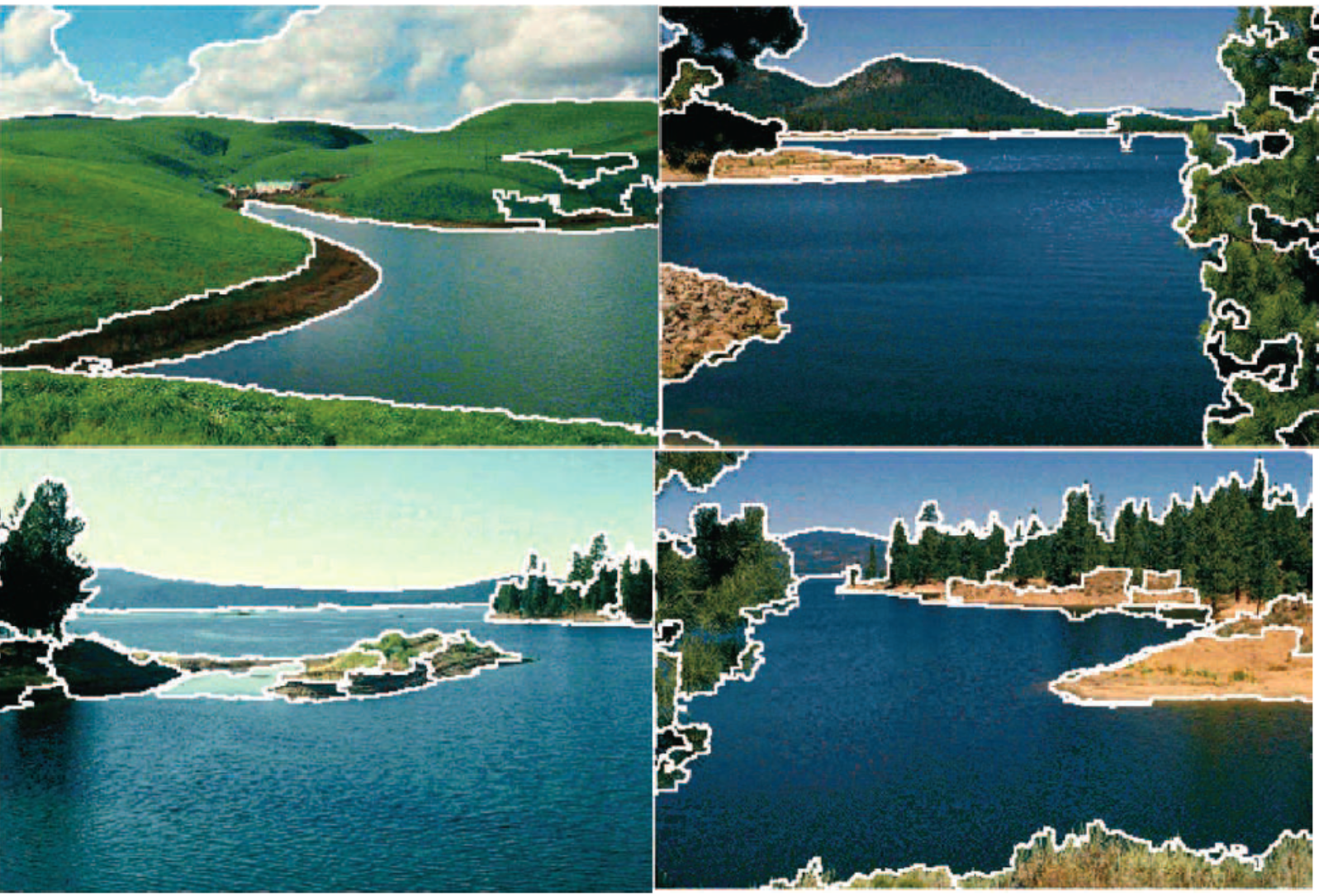
From doi: 10.1109/34.1000236 Find segments in an image of your choice using mean shift. For each pixel, define five features: x and y positions, luminosity, and color channels (U, V). Luminosity and U, V color channels (YUB color encoding) is a different representation of an image than RGB. To create a YUB encoding from RGB, weighted values of R, G, and B are summed to produce Y, a measure of overall brightness or luminance. U and V are computed as scaled differences between Y and the B and R values. The formula to convert RGB to YUB is as follows. Note that for the constants below, RGB is normalized between 0 and 1, meaning you will have to divide RGB values by 256.
  Y = 0.299R + 0.587G + 0.114B
  U = 0.492 (B-Y)  # or U = -0.147R - 0.289G + 0.436B
  V = 0.877 (R-Y)  # or V = 0.615R - 0.515G - 0.100B
The inverse conversion is with these formulas:
   R = Y + 1.140V
   G = Y - 0.395U - 0.581V
   B = Y + 2.032U
Create a new image where each pixel has the RGB values of the centroid.