- Convolutional neural networks (CNNs) are specifically suitable for working with image input data. But they can also be used for other data input.
- CNNs’ strength is in their pattern detection in images. Patterns in an image are edges (sharp changes in luminosity or color), shapes, and objects.
- Their difference from standard neural networks is the convolutional hidden layers that they have in addition to standard layers. A typical layer in a neural network receives data from its previous layer, transforms the data, and hands them to the next layer. A convolutional layer does similarly, except that the kind of transformation it does is a convolution.
- There are different convolutional layers that detect different patterns, e.g. edges, corners, squares, and circles, depending on how deep the layer is.
What is convolution
- A convolutional layer in a NN uses a filter to transform the input. A filter is as a small matrix, e.g. \(3 \times 3\), initialized with random values. The true values will be learned by the network. At each iteration of the network, the filter slides across all pixels and creates a new set of pixels.
- This excel file shows how a filter can detect edges.
Why using convolution instead of a fully connected network?
Reducing the number of shared parameters by parameter sharing
If we have an image of size \(48 \times 48 \times 3\), where 3 is for RGB values, there are 6,912 input values. A convolution with two \(3 \times 3\) filters will create a new layer with size \(46 \times 46 \times 2 = 4232\). Connecting two layers with these sizes in a fully connected way means we would have more than 29 million parameters to learn, only between two layers. That is too many parameters for a small image like this. But using a convolution step, we only have 56 parameters to learn (two filters each with 27 elements and one bias term). The reason behind this reduction in parameter space is that we use the same feature detector (e.g. vertical edge detector), and hence the same parameters, every time we slide across the picture.
Reducing the number of shared parameters by having sparse connections
In a convolutional layer, each new pixel depends only on a small number of pixels from the previous layer, i.e., only those on which the filer was applied. The rest of the pixels do not affect the new pixel. This helps reduce the number of parameters.
Padding
- In the simple convolution, the dimension of the output matrix will be smaller than the input. Specifically, if the input had \(n \times n\) dimensions, and the filter has \(f \times f\) dimensions, the output will have \((n-f+1, n-f+1)\) dimensions. Hence, a \(7 \times 7\) matrix will turn into a \(5 \times 5\) matrix when a \(3 \times 3\) is applied to it.
- Applying convolution like this several times, will reduce the image size too small. Additionally, information on the edges are discarded.
- To solve these problem, we can add padding to the input with an additional border of zeros.
Striding
- Striding is by how much the sliding window moves at a time (step size). Normally it moves one cell at a time (stride=1), but it is possible to jump further.
- Having a stride larger than 1 results in the output becoming smaller than the input. This is called downsampling. With downsampling we lose of the information in the image but we end of with a smaller input and hence improve computation cost.
- Each dimension of the output size when having padding and striding, is governed by the following formula: \(\frac{n+2p-f}{s} + 1\), where n is a dimension size of the input, f is a dimension size of the filter, p is padding, and s is stride length. If the formula does not return an integer, it should be rounded down (
floorfunction in Julia). From the implementation perspective, rounding down means that convolution is only applied when filter is fully overlapping part of an image.
Convolution over volumes
- When the input, e.g. an image, is not 2 dimensional (gray scale), but 3 dimensional (RGB), our filter should also be 3D.
- To apply the filter, multiply each element of the filter to each element of the corresponding section of the input. Add up all the values to create a new value for the output. So although the input and the filter are 3D, the output will still remain 2D.
Pooling layer
- A pooling layer reducing the size of features to improve performance and also make some features more robust.
- Pooling operation is similar to a convolution. We slide a filter with a filter size across and stride across a matrix. But instead of doing a dot product, we just choose the maximum or the mean value and record it as output. In pooling, we choose a single value from a given region using a max or mean function, whereas in convolution we do a dot product of filter values to that region. This means that the filter values are learned, whereas in pooling there is no learning. Pooling is a simple downsampling procedure.
- When pooling, we do not use padding because our intention is to reduce dimensions.
One layer of convolution in the network
- Say we have an image with dimensions \(10 \times 10 \times 3\), where 3 is for the three RGB channels. We want to apply two different filters on the image, each of which with dimensions \(3 \times 3 \times 3\), where the last 3 is again for the three channels RGB. The output of sliding each filter on the image will be of dimensions \(8 \times 8\) (assuming padding is 0 and stride is 1). Now, this output needs to be nonlinearized. To that end, we first add a bias \(b\) to each element. This is similar to how we had a bias term in linear regression (\(y = ax + b\)). After that, we apply a nonlinearizing function, such as ReLu to each element. The output will keep its dimensions. Since we had two filters applied to the image, the final output of this convolution layer will have dimensions \(8 \times 8 \times 2\).
- If you want to use a fully connected layer after a convolution layer, for example, as a regression output layer, you can just flatten the convolution layer into a vector.
- Why would we use multiple filters at the same time? To detect multiple features, e.g. horizontal and vertical and diagonal edges, at the same time.
- An important decision in designing convolutional neural networks is deciding the number of filters and padding and striding for each layer. A general trend is to keep the dimensions similar to the image for a few layers, and then gradually reduce the size of height and width dimensions while increasing the depth. Examples of successful structures are LeNet-5, AlexNet, and VGG16.
Notable architectures
- LeNet-5: This architecture is an old one that is designed for hand written or machine printed character recognition. Input images are gray scale (\(32 \times 32 \times 1\)).

-
AlexNet: Proposed in 2012 by Alex Krizhevsky, is still a popular network architectures. The architecture was used in the ImageNet Large Scale Visual Recognition Challenge to classify 1.2 million images into more than a thousand categories.
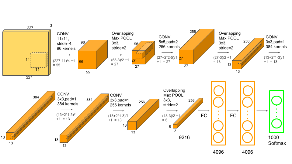
Input images are of size \(227 \times 227 \times 3\) and it network has more than 60 million parameters to learn.
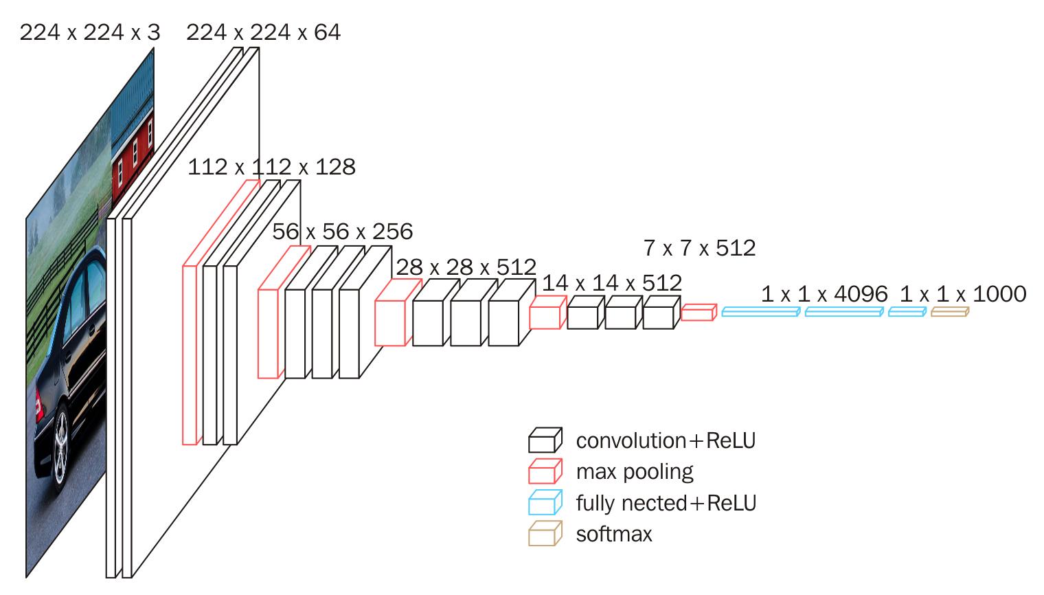
- VGG16: Proposed in 2014 by Karen Simonyan & Andrew Zisserman, VGG16 is another popular network architecture. This structure was used in the ImageNet 2014 challenge.
Data augmentation
- Computer vision is a complex task. Training the models requires large amount of data. Depending on the task, you may not have enough data to train your model confidently. Data augmentation is a common practice in computer vision. We can create more images from the ones we have, using the methods below.
- Mirroring.
- Random cropping. The crops should not be too small.
- Color shifting. Adding values from RGB channels. For example, we can add [-20, 20, -20] to RGB.
- Rotation.
- Sheering.
Exercises
- Do the exercises in this notebook
- Write a LeNet-5 model with Flux to classify written digits.
Here is an example of how a CNN is built with Flux:
using Flux, Statistics
using Flux: onehotbatch, onecold, logitcrossentropy
using MLDatasets

train_x, train_y = MNIST.traindata()
test_x,  test_y  = MNIST.testdata()

lr = 3e-3
epochs = 20
batch_size = 128
imgsize = (28,28,1)
cnn_output_size = Int.(floor.([imgsize[1]/8,imgsize[2]/8,32]))

model = Chain(
  # First convolution, operating upon a 28x28 image
  Conv((3, 3), imgsize[3]=>16, pad=(1,1), relu),
  MaxPool((2,2)),

  # Second convolution, operating upon a 14x14 image
  Conv((3, 3), 16=>32, pad=(1,1), relu),
  MaxPool((2,2)),

  # Third convolution, operating upon a 7x7 image
  Conv((3, 3), 32=>32, pad=(1,1), relu),
  MaxPool((2,2)),

  # Reshape 3d array into a 2d one using `Flux.flatten`, at this point it should be (3, 3, 32, N)
  flatten,
  Dense(prod(cnn_output_size), 10),
  softmax
)

cost(x, y) = logitcrossentropy(model(x), y)

# https://fluxml.ai/Flux.jl/stable/training/optimisers/#Optimiser-Reference
opt = ADAM()
The model can then be trained using
Flux.train!.