Linear algebra

Linear Algebra is a cornerstone for machine learning algorithms. It helps us analyze linear equations with lots of variables without getting lost. An example of such linear equation systems is a price list. Suppose you have the total price of a shopping list with two items: apples and oranges. But you do not have the price of each item separately. One day, you buy 3 apples and 2 oranges and it costs CHF 10. The other day you buy 5 apples and 3 oranges and it costs CHF 15. You can write these two prices as two linear equations:

Writing and solving by hand many of these equations can be hard. We can write these equations as a matrix problem and let the computer solve them from a general case:

Another kind of problems that we can solve with linear algebra are optimization problems where we want to find the parameter values of an equation that best fit the data that we observe. This task is generally speaking what machine learning and neural network algorithms do.

Take the following plot of car weight vs displacement for different makes. Displacement is the volume of all the pistons inside the cylinders. Could we fit a line or curve to these data to make predictions?

We will solve similar questions during this course.

Vectors

• Vectors can be thought of in a variety of different ways - some geometrically, some algebraically, some numerically. This allows vectors to be applied to a lot of problems. For example, vectors can represent something that moves in a space of fitting parameters, or position in three dimensions of space and in one dimension of time, or a list of numbers.
• In computer science, vector is a list of attributes of an object, whereas in physics, it shows the direction of movement.
• The performance of a model can be quantified in a single number. One measure we can use is the Sum of Squared Residuals, SSR. It files all of the residuals (the difference between the measured and predicted data), square them and add them together.
• The goal in machine learning is to find the parameter set where the model fits the data as well as it possibly can. This translates into finding the lowest point, the global minimum, in this space.
• Often we can’t see the whole parameter space, so instead of just picking the lowest point, we have to make educated guesses where better points will be. We can define another vector, \(\Delta p\), in the same space as \(p\) that tells us what change can be made to \(p\) to get a better fit.
• When a vector is represented by two numbers in the coordinate system, rather than two pairs, then it is assumed that the start of the vector is the center of the coordinate system.

Exercise

A linear line has the equation \(y = ax + b\) where \(a\) is called a coefficient and \(b\) is the intercept.

Write a function called predict so that it accepts three parameters: x, a, and b, all of which are if type Real. After that, create a scatter plot with the Weight_in_lbs column of the car dataset in the x-axis and the Displacement column in the y-axis. Add a line to this scatter plot whose x-axis values are Weight_in_lbs and the y-axis values are from the predict function.

Try different a and b values to find a good fit by eye. This is a task that we will learn to automate and find good parameters to fit the data. When the data are high-dimensional we won’t be able to test the fit by eye.

What set of parameters seem to have the smallest SSR?

using VegaDatasets
using DataFrames

car = DataFrame(dataset("cars"));

Operations

• Scalar operations: \(\begin{pmatrix} 1\\ 2 \end{pmatrix} + 2 = \begin{pmatrix} 3\\ 4 \end{pmatrix}\)
• Elementwise operations: \(\begin{pmatrix} a_1\\ a_2 \end{pmatrix} + \begin{pmatrix} b_1\\ b_2 \end{pmatrix} = \begin{pmatrix} a_1 + b_1\\ a_2 + b_2 \end{pmatrix}\)
• \(r + s = s + r\). Think of it as geometrical addition of two vectors.
• Associative \(t + (s + r) = (t + s) + r\).

Inner or dot product

Calculate length and directions

• The length of a vector is given by the hypotenuse (Pythagoras). If \(r = [a, b]\), then the size of \(r\) is \(\| r \| =\sqrt{a^2 + b^2}\). But the definition applies to higher dimensions too. The length of any vector is the square root of sum of squares of its elements.
• The dot product of two vectors is a single number (scalar): \(r.s = \sum_{i=1}^{n} r_i s_i\)

Properties of dot product

1. Commutative: \(r.s = r.s\)
2. Distributive over addition: \(r.(s+t) = r.s + r.t\)
3. Associative: \(r.(as) = a(r.s)\), where a is a number (scalar).

The link between the dot product and its length

• The dot product of a vector to itself is the square of its length: \(r.r = {r_1}^2 + {r_2}^2 = \|r\|^2\).

Cosine and dot product

• Cosine rule: in a triangle with sides \(a\), \(b\), and \(c\), \(c^2 = a^2 + b^2 - 2ab \cos(\theta)\), where θ is the angle between \(a\) and \(b\). If θ is 90, then cos(90)=0, and we derive Pythagoras.
• From the cosine rule, it can be derived that: \(r.s = \|r\| \|s\| cos(\theta)\). The dot product of two vectors is the product of their length times the cos of their angel. If θ = 90, cos(θ)=0 and the dot product is 0. If they are pointing in the same direction, then their dot product equals the product of their lengths. If they are in opposite directions, \(\cos(180) = -1\), their dot product is minus their lengths product.

Projection

• \(r.s = \|r\| * projection(s)\), where \(projection(s) = \|s\| \cos(\theta)\) is the scaler projection of s onto r because \(\cos(\theta)\) is the adjacent over the hypotenuse. This is if r and s are two vectors with the same start and θ is the angle between them. The scaler projection is the the size of the “shadow” of s over r if there was a light perpendicular to r. To get the vector projection, that is, the vector resulting from projecting s on r, we multiply the scaler projection by \(\frac{r}{\|r\|}\).

Matrices

• A matrix times a vector, transforms the vector. If you multiply a matrix by the unit vector, it is as if you are transforming the space (basis).

Types of matrix transformation

• Identity matrix: it consists of the unit vectors (diagonal) and changes nothing.
• You can transform the coordinates in any linear way you want by choosing the right matrix.
• Inverse matrix: a matrix that returns the identity matrix when multiplied to a matrix.

Solving series of equation

• If you have n equations and n variables, you can write them in the form of \(A\times r = s\), where A is a matrix of coefficients, r is a vector of variables, and s is a vector of results.
• If you multiply both sides of the equation by \(A^{-1}\) (inverse of A), then on the left side you will have \(I \times r\) which equals r, and on the right side \(A^{-1} \times s\). So you have found r, the variables.

Determinants and inverses

• The determinant is a scalar value that can be computed from the elements of a square matrix and is denoted det(A), det A, or \(\lvert A \rvert\). Geometrically, it can be viewed as the volume scaling factor of the linear transformation described by the matrix, that is, by how much the matrix stretches or shrinks the space. For example, if matrix \(2I\), where \(I\) is the identity, transforms a square to 4 times its size. The determinant of \(2I\) is therefore 4. This works in any direction.

Changing basis

• Say we have basis \(U\) and \(V\). The unit vectors of basis \(V\) in basis \(U\) are [3,1] and [1,1]. To to convert the coordinates of a vector \(B\), which is in basis \(V\), to basis \(U\), we have to multiply the \(V\)’s basis matrix ([3,1; 1,1]) to the vectors coordinates. That will give the coordinates of \(B\) in basis \(U\). But what if we want to translate basis \(U\) to basis \(V\)? We can inverse the \(V\) matrix. That will be the coordinates of \(U\) in \(V\)’s world.
• An easier way to change basis of a vector is using dot products. If \(U\) and \(V\)’s vectors are orthogonal, you can use projections. To find the coordinates of a vector \(v\) in a new basis that consists of \(b_1\) and \(b_2\), find the component of \(v\) on \(b_1\) and \(b_2\). The component of \(v\) on \(b_1\) is \(\frac{v.b_1}{\|b_1\|^2}\) and the component of \(v\) on \(b_2\) is \(\frac{v.b_2}{\|b_2\|^2}\). The two components together give the new coordinates of v.

Eigenvalues and eigenvectors

• When you transform a space by multiplying a matrix to it, there are some vectors in that space that remain on the same span after the transformation. Those vectors are eigenvectors. However, the eigenvectors can change their direction or length. The change in their length is represented by eigenvalues.
• How to formally define them? \(Ax=\lambda x\), where A is matrix, λ is a scalar (eigenvalue), and \(x\) is a vector, the eigenvector. The equation says that the transformation matrix times a vector equals a the same vector times a scalar, meaning that the vector is in the same span.
• Another formulation is \((A - \lambda I)x = 0\). We need the identity matrix here because matrix subtraction from a scalar is not defined. Since x=0 is a trivial solution, we are interested in finding the solution to \(A - \lambda I=0\) so \(det(A-\lambda I) = 0\).

Exercises

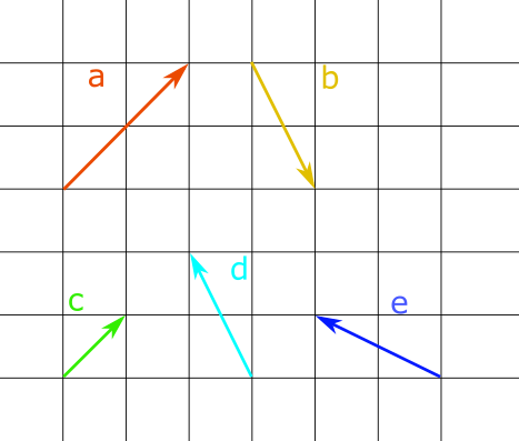
1. Given the diagram above and considering that all vectors start from [0,0]:
   1. What is the numerical representation of the vector \(a\)?
   2. Which vector in the diagram corresponds to \([-1, 2]\)?
   3. What is the numerical representation of \(2c\)?
   4. What is the numerical representation of \(-b\)?
   5. What is the sum of vectors \(d\) and \(e\)?
2. Say we have vector r = [1,2,3,4] and s = [5,6,7,8].
   1. What is the size of the vector r and s?
   2. What is the inner product of s and r?
   3. What is the projection of s on r, and the projection of r on s?
   4. What is the angel between r and s?
3. Check whether the angel between \(b_1 = [1, 1]\) and \(b_2 = [1, -1]\) is 90 degrees.
4. Download an image and try to rotate it with a rotation matrix, e.g. [-1 1; 1 1]. An image is a matrix of pixels, where each pixel is an RGB type that has three values for Red, Green, and Blue. To apply a transformation matrix to an image, you need to apply it to each pixel position, and find its new position after the transformation. Then save the value of the pixel from the original image in a new matrix. Using Pluto for this task is recommended because you can see the image without saving it.

   using Images
   using ImageMagick
   using FileIO
   
   img_path = "someimage.jpg"
   img = load(img_path)